
No Limitation
[개념+코드 개인 공부 용] A Simple Framework for Contrastive Learning of Visual Representations 본문
[개념+코드 개인 공부 용] A Simple Framework for Contrastive Learning of Visual Representations
yesungcho 2023. 11. 25. 18:14Contrastive learning에서 잘 알려져있는 SimCLR 논문으로 개념 및 코드 위주로 정리하고자 합니다.
코드는 Pytorch 기반으로 Janne님의 github 링크를 바탕으로 분석하였습니다.
https://github.com/Spijkervet/SimCLR/tree/master
GitHub - Spijkervet/SimCLR: PyTorch implementation of SimCLR: A Simple Framework for Contrastive Learning of Visual Representati
PyTorch implementation of SimCLR: A Simple Framework for Contrastive Learning of Visual Representations by T. Chen et al. - GitHub - Spijkervet/SimCLR: PyTorch implementation of SimCLR: A Simple Fr...
github.com
개념부터 찬찬히 살펴보겠습니다.
1. Abstract
논문에는 다음과 같이 정리가 되어 있습니다.
- Composition of data augmentations plays a critical role in defining effective predictive tasks
즉, Contrastive Learning을 하기 위해, data augmentation 기법이 굉장히 효과적이었다는 것을 언급하고 있습니다.
- Introducing a learnable nonlinear transformation between the representation and the contrastive loss substantially improves the quality of the learned representations
그대로 설명하면 Learnable한 nonlinear transformation을 contrastive loss에 도입하는 것이 매우 강력한 representation power를 낳았다고 합니다. 사실 어려워보이지만 별 거는 아닌게 contrastive learning을 위해 일종의 projection-head을 구축한 것을 의미합니다. backbone을 통과한 feature에서 nonlienar transformation을 수행하는 linear layer를 더 붙여서 뽑아낸 feature가 일반적인 backbone을 통과한 feature 보다 더 contrastive learning이 잘 수행되었음을 의미합니다. 아무래도 learnable parameter를 더 사용하니까 그렇겠죠.
- Contrastive learning benefits from larger batch sizes and more training steps compared to supervised learning
또한 큰 batch size를 사용하고 많은 training step을 밟는 것이 굉장히 중요하다고 언급하고 있습니다. 이는 과거의 Memory bank 라는 방법을 사용해서 수행되었던 contrastive learning의 한계점을 보완한 것과 관련이 있습니다.
그럼 본격적으로 내용을 살펴보겠습니다.
2. Methodology
The Contrastive Learning Framework
본문에 나와있는 다음 문장은 SimCLR의 핵심을 설명한다고 할 수 있습니다.
"SimCLR learns representations by maximizing agreement between differently augmented views of the same data example via a contrastive loss in the latent space."
즉, 예를 들어 $x_i$ 라는 이미지가 있다고 할때, 이를 augmentation을 수행한 $x_j$가 있다고 해보겠습니다. 아무리 우리가 weak, strong augmentation을 적용해도 결국 $x_i$ 랑 $x_j$는 같은 맥락을 담고 있는 정보임을 알 수 있습니다. 즉, 둘은 positive pair가 되는 것이죠. 이러한 특징을 활용한 전략이 바로 SimCLR의 기본 아이디어 입니다.
보다 개념적으로는 아래 그림과 같습니다.

예를 들어, 강아지 사진을 기준으로 설명하면 왼쪽 열은 original image들 $N$개, 오른쪽 열은 augmented (여기선 color jitter)된 이미지들 $N$개를 의미합니다. 자 그럼 강아지 사진을 기준으로는 $x_i$ 나 $x_j$는 같은 강아지를 의미합니다. 즉, positive pair를 의미합니다. 하지만 그 외의 나머지 $2(N-1)$개의 이미지들은 전부 negative pairs들이 됩니다. 이런 특징을 가지고 모형을 학습하는 전략을 SimCLR는 사용합니다.
그럼 어떻게 contrastive learning을 수행하는 지를 아래 그림과 더불어 같이 살펴보겠습니다.

우선 $\widetilde{x}_{i}$는 본래 $x$, $\widetilde{x}_{j}$는 augment 이미지를 의미합니다. 본 논문에서는 ResNet18 네트워크를 사용하였으며 average pooling layer 이후부터 싹 제거하여 그 전까지 네트워크를 통과한 feature $h_{i},h_{j}$를 뽑아내는 feature etraction $f(.)$ 를 정의합니다. 다음으로 이 $h_{i}, h_{j}$를 그대로 사용하는 것이 아니라 별도의 linear layer들로 구성된 projection head $g(.)$를 사용하여 최종적으로 $z_{i}, z_{j}$를 도출합니다. 이는 다음과 같이 일반적인 non-linear transformation 구조를 따릅니다.

이 녀석들을 기준으로 contrastive learning을 수행합니다. 논문에서는 projection head를 통과한 128 사이즈의 1-dim vector를 추출했다고 하는데 이는 구현체마다 다르게 설정하는 것 같습니다. 밑에서 실습할 코드에서는 64 사이즈를 사용하였습니다.
그리고 저 $z_{i}, z_{j}$를 바탕으로 NT-Xent (Normalized Temperature-scaled cross'X' ENTropy loss) 를 사용해서 contrastive learning을 수행합니다.
이를 직관적으로 그림으로 표기하면 아래와 같습니다.

자 그러면 저 우측 아래의 NT-Xent loss에 대해 구체적으로 살펴보겠습니다.
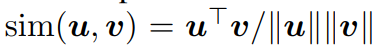
저기서 $sim$의 경우 두 벡터 간의 유사도를 계산하는 함수를 의미하는데, 이전 InfoNCE loss의 경우 여기를 log-bilinear model을 활용해서 공유 정보를 계산했었습니다. 반면 NT-Xent의 경우 cosine similarity를 사용합니다.
그리고 중간에 $\tau$ 가 들어가 있는데 이는 temperature라는 parameter로서 흔히 contrastive loss에서 sensitivity를 regularizes할 때 사용되는 파라미터입니다. 즉, 학습을 안정적으로 수행되게 해주는 파라미터를 의미하고, 실제로 논문에서는 이 적절한 $\tau$을 고르기 위해 많은 실험을 수행합니다.
즉, 이 NT-Xent를 활용하여 학습을 수행하는 슈도 코드는 아래와 같습니다.
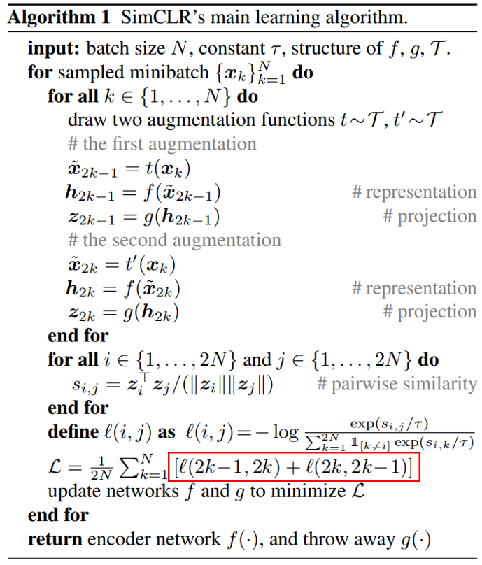
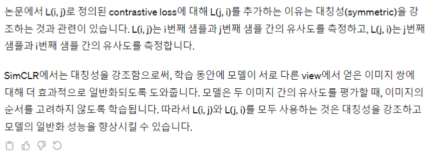
다만 궁금한 점이 위에 표시한 빨간 박스처럼, loss function을 $l$이라고 하면, 여기서 계산을 $l(i,j)$도 하고 $l(j,i)$도 수행합니다. cosine similarity는 교환법칙이 성립하는 것으로 아는데 이렇게 함수를 구성한 이유가 있는지는 개인적으로 궁금합니다. 별도의 논문에는 언급은 없고 ChatGPT는 "대칭성" 때문이라고 언급을 하는데, 잘 이해는 안갑니다.. ㅠ 혹시 아시는 분은 댓글 부탁드립니다..ㅠ
Training with Large Batch Size
또한 논문에서는 큰 Batch size를 사용한 것이 이점이 있다고 언급을 합니다.
"To keep it simple, we do not train the model with a memory bank. Instead, we vary the training batch size N from 256 to 8192."
보면 큰 배치 사이즈 사용함으로써 Memory bank라는 기법을 사용하지 않고도 모형이 안정적인 contrastive learning을 수행할 수 있었다고 언급합니다.
우선 Memory bank라는 것은 네트워크가 학습한 모든 표현(representations)들을 저장해놓고 그때 그때 마다 랜덤 샘플링을 통해 contrastive learning에 사용하는 방법으로 SimCLR 이전에 많이 사용된 방법이라고 합니다 (여기 부분에 있어서는 아직 공부가 덜 되 공부를 더 해야할 거 같습니다 ㅠ). 하지만 이 방법은 많은 메모리 손실에, 네트워크가 한참 업데이트한 뒤에 예전에 저장된 representation을 사용하는 것은 일관성이 없다는 한계점이 존재했다고 합니다. 이 문제를 극복하기 위해 SimCLR에서는 거대한 batch size를 사용해 굳이 memory bank에 저장할 필요 없이도 충분한 배치 사이즈를 통해 다양한 negative pairs들을 사용함으로써 강건한 contrastive learning이 가능하다고 주장합니다.
하지만 이런 거대한 batch size를 사용하게 되면 (심지어 8000까지..) 모형의 iteration이 돌아가는 횟수가 필연히 줄 수 밖에 없죠. 그러면 학습이 충분히 되기 위해 큰 learning rate을 사용할 수 밖에 없는데 그러면 모형이 안정적으로 global optima를 찾는데 어려움을 겪게 되는 문제점이 있습니다. 이를 극복하기 위해 논문에서는 LARS Optimizer라는 개념을 사용합니다. 이 LARS Optimizer는 큰 배치와 큰 learning rate를 사용할 때에도 안정적인 학습을 수행할 수 있게 돕는 optimizer를 의미하는데, 이 부분에 대해서는 추후에 정리하도록 하겠습니다.
LARS Optimizer original paper
You et al., 2017, Large Batch Training of Convolution Networks
https://arxiv.org/abs/1708.03888
자 그럼 위의 방법이 어떻게 코드로 Running이 되는지 하나씩 살펴보겠습니다.
3. Code Implementation
코드는 크게 3가지 파트를 정리하고자 합니다.
- Augmentation 코드 파트, 2N개의 batch sample 생성
- SimCLR 아키텍처, projection-head 구성
- NT-Xent loss function 함수 및 전체 돌아가는 코드 분석
[1] Augmentation을 통해 $x_i$ (본데이터), $x_j$ (augment 데이터)를 구축하는 부분
우선 논문에서는 데이터의 경우 ImageNet ILSVRC-2012 데이터셋과 CIFAR-10 데이터셋을 사용했는데 우리는 ImageNet ILSVRC-2012 데이터셋을 바탕으로 코드를 running 해보았습니다.
우선, 아래와 같이 데이터셋을 구축할 때 augmentation pair 쌍을 구축하기 위해 아래와 같이 augmentation을 수행합니다.
train_dataset = torchvision.datasets.STL10(
            "./datasets",
            split="unlabeled",
            download=True,
            ### 이 부분이 augmentation (transform)을 수행하는 부분
            transform=TransformsSimCLR(size=224),
        )
구체적으로는 TransformsSimCLR는 아래와 같이 구성됩니다.
class TransformsSimCLR:
    def __init__(self, size):
        s = 1
        color_jitter = torchvision.transforms.ColorJitter(
            0.8 * s, 0.8 * s, 0.8 * s, 0.2 * s
        )
        ### 학습 데이터의 경우,
        ### (1) Resize -> (2) Horizontal Flip -> (3) Color Jitter -> (4) Grayscale
        ### 다음 단계가 랜덤으로 수행이 됨
        self.train_transform = torchvision.transforms.Compose(
            [
                torchvision.transforms.RandomResizedCrop(size=size),
                torchvision.transforms.RandomHorizontalFlip(),  # with 0.5 probability
                torchvision.transforms.RandomApply([color_jitter], p=0.8),
                torchvision.transforms.RandomGrayscale(p=0.2),
                torchvision.transforms.ToTensor(),
            ]
        )

        ### 테스트셋의 경우 예측을 위한 resize만 적용함
        self.test_transform = torchvision.transforms.Compose(
            [
                torchvision.transforms.Resize(size=size),
                torchvision.transforms.ToTensor(),
            ]
        )

    def __call__(self, x):
        return self.train_transform(x), self.train_transform(x)
즉, 코드 상에서는 여러 가지 augmentation 전략을 수행한 것을 확인할 수 있습니다.
train_sampler = None
train_loader = torch.utils.data.DataLoader(
        train_dataset,
        batch_size=128,
        shuffle=(train_sampler is None),
        drop_last=True,
        num_workers=8,
        sampler=train_sampler,
    )
(x_i, x_j), _ = next(iter(train_loader))

x_i ## size is [128,3,224,224] 128 is batch size
x_j ## size is [128,3,224,224] 128 is batch size

import matplotlib.pyplot as plt
plt.imshow(x_i[0].detach().cpu().numpy().transpose((1,2,0)))
import matplotlib.pyplot as plt
plt.imshow(x_j[0].detach().cpu().numpy().transpose((1,2,0)))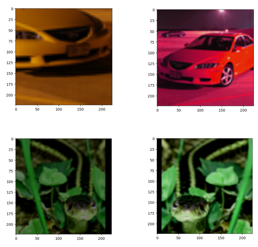
저 샘플들은 아무리 augmentation을 수행했다 하더라도, positive pair라는 것을 알 수 있습니다. (같은 차, 뱀이므로)
또한 코드 상에서도 알 수 있듯, 우리는 batch 사이즈로 128 ( Large batch를 사용했다는 것에 주목 ), 이미지 사이즈는 224로 설정하였습니다.
자 다음으로, SimCLR 네트워크를 구축하는 부분을 살펴보겠습니다.
[2] SimCLR 아키텍처, projection-head 구성
리마인드해보면 우리는 ResNet18 네트워크를 사용하였으며 backbone $f(.)$을 통과한 feature map $h$가 있었고, 이를 다시 contrastive learning에 사용할 vector로 전환하기 위해 projection head $g(.)$를 구축했었습니다. 실제로 이는 매우 간단하게 구현되어 있는데 아래 코드를 살펴보겠습니다.
def get_resnet(name, pretrained=False):
    resnets = {
        "resnet18": torchvision.models.resnet18(pretrained=pretrained),
        "resnet50": torchvision.models.resnet50(pretrained=pretrained),
    }
    if name not in resnets.keys():
        raise KeyError(f"{name} is not a valid ResNet version")
    return resnets[name]

## 사용할 backbone 추출, scratch로 사용
encoder = get_resnet("resnet18", pretrained=False)
## 여기서 n_features는 512 사이즈이고 이를 바탕으로 projection head를 구축한다.
n_features = encoder.fc.in_features  # get dimensions of fc layer
위 backbone (encoder)를 바탕으로 projection-head까지 구축한 최종 SimCLR 모델 코드를 살펴보겠습니다.
class SimCLR(nn.Module):
    def __init__(self, encoder, projection_dim, n_features):
        super(SimCLR, self).__init__()

        self.encoder = encoder
        self.n_features = n_features

        # Replace the fc layer with an Identity function
        self.encoder.fc = Identity()

        # We use a MLP with one hidden layer to obtain z_i = g(h_i) = W(2)σ(W(1)h_i) where σ is a ReLU non-linearity.
        ## 바로 이 부분이 projection-head가 된다.
        ## 512 사이즈의 vector를 입력으로 받아 최종 'projection_dim' 사이즈의 output vector를 도출한다.
        self.projector = nn.Sequential(
            nn.Linear(self.n_features, self.n_features, bias=False),
            nn.ReLU(),
            nn.Linear(self.n_features, projection_dim, bias=False),
        )

    def forward(self, x_i, x_j):
        h_i = self.encoder(x_i)
        h_j = self.encoder(x_j)

        z_i = self.projector(h_i)
        z_j = self.projector(h_j)
        return h_i, h_j, z_i, z_j
        ## 최종적으로 SimCLR 모형은 다음과 같은 h_i,h_j, z_i, z_j를 도출
        ### 우리는 contrastive learning을 위해, 즉 NT-Xent loss를 도출하는 데에는 z_i, z_j를 사용

## 앞에서 구한 n_features를 사용
model = SimCLR(encoder, 64, n_features) ## 여기서는 projection head size로서 64를 사용, 논문 상 128
device = torch.device('cuda')
model = model.to(device)
마지막으로 NT-Xent loss가 구성된 부분을 살펴보겠습니다.
[3] NT-Xent Loss
자 이제 저렇게 구성한 모형을 바탕으로 contrastive learning을 수행하는데 이때 사용되는 loss가 바로 NT-Xent입니다.
우선 아래 큰 train 함수의 구성을 살펴보겠습니다.
criterion = NT_Xent(batch_size=128, temperature=0.5, world_size=1)
### 여기서 temperature는 일종의 학습의 안정성과 수렴 속도 등을 규제하는 regulator로 논문에서는
### 적합한 temperature를 선정하기 위해 여러 실험을 수행한다. 여기서는 simple하게 0.5로 주었다.

### 우리는 별도의 분산 처리는 적용하지 않았으므로 world_size는 1로 설정하였다.

### train() 함수의 일부분을 살펴보자
loss_epoch = 0
for step, ((x_i, x_j), _) in enumerate(train_loader):
    optimizer.zero_grad()
    x_i = x_i.cuda(non_blocking=True)
    x_j = x_j.cuda(non_blocking=True)

    # positive pair, with encoding
    h_i, h_j, z_i, z_j = model(x_i, x_j)

		# 바로 여기! 저 위의 NT_XENT는 어떻게 구성되는 걸까?
    loss = criterion(z_i, z_j)
    loss.backward()

    optimizer.step()
결국 핵심은 위에서 정의된 criterion() 함수인 NT-Xent loss가 어떻게 동작하는 지를 살펴보아야 합니다. 우선 loss 전체를 살펴보겠습니다.
class NT_Xent(nn.Module):
    def __init__(self, batch_size, temperature, world_size):
        super(NT_Xent, self).__init__()
        self.batch_size = batch_size
        self.temperature = temperature
        self.world_size = world_size

        ### 우선 여기 mask라는 것을 정의한다.
        self.mask = self.mask_correlated_samples(batch_size, world_size)
        self.criterion = nn.CrossEntropyLoss(reduction="sum")
        ### Contrastive Learning을 위해서는 similarity score가 필요한데 NT-Xent에서는 cosine similarity를 사용한다
        self.similarity_f = nn.CosineSimilarity(dim=2)

    def mask_correlated_samples(self, batch_size, world_size):
        N = 2 * batch_size * world_size
        mask = torch.ones((N, N), dtype=bool)
        mask = mask.fill_diagonal_(0)
        for i in range(batch_size * world_size):
            mask[i, batch_size * world_size + i] = 0
            mask[batch_size * world_size + i, i] = 0
        return mask

    def forward(self, z_i, z_j):
        """
        We do not sample negative examples explicitly.
        Instead, given a positive pair, similar to (Chen et al., 2017), we treat the other 2(N − 1) augmented examples within a minibatch as negative examples.
        """
        N = 2 * self.batch_size * self.world_size

        ### 우리는 분산처리를 하지 않았으니 여기는 무시
        if self.world_size > 1:
            z_i = torch.cat(GatherLayer.apply(z_i), dim=0)
            z_j = torch.cat(GatherLayer.apply(z_j), dim=0)

        z = torch.cat((z_i, z_j), dim=0)

        sim = self.similarity_f(z.unsqueeze(1), z.unsqueeze(0)) / self.temperature

        sim_i_j = torch.diag(sim, self.batch_size * self.world_size)
        sim_j_i = torch.diag(sim, -self.batch_size * self.world_size)

        # We have 2N samples, but with Distributed training every GPU gets N examples too, resulting in: 2xNxN
        positive_samples = torch.cat((sim_i_j, sim_j_i), dim=0).reshape(N, 1)
        negative_samples = sim[self.mask].reshape(N, -1)

        labels = torch.zeros(N).to(positive_samples.device).long()
        logits = torch.cat((positive_samples, negative_samples), dim=1)
        loss = self.criterion(logits, labels)
        loss /= N
        return loss
상당히 복잡해보이는데 뜯어보면 사실 크게 복잡한 것은 없습니다. 하나씩 line by line으로 살펴보겠습니다.
우선, 위의 mask_correlated_samples 함수부터 뜯어보겠습니다.
### 우선 batch_size는 128로 설정하였고 world_size는 1이므로, 여기서 N은 batch 의 2배인 256이 된다.
N = 2 * batch_size * world_size

### mask는 우선 1 (True, dtype=bool이므로) 로 채워져있는 (256,256) matrix가 된다.
mask = torch.ones((N, N), dtype=bool)

### 다음으로 해당 마스크에서 주대각선 성분은 전부 0으로 채운다
mask = mask.fill_diagonal_(0)
이 'mask'라는 것을 가시화해보면 아래와 같습니다.
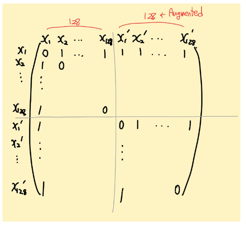
여기 매트릭스처럼, 처음에 $x_{1}, x_{2}, …, x_{128}$이 존재하고, 이것의 augmented 버전이 $x'_{1}, x'_{2}, …, x'_{128}$이 존재하여 총 256개의 샘플이 존재하고 이 벡터가 구축한 행렬 mask의 주대각선 성분을 0으로 하면 위의 그림과 같이 구성됩니다.
여기서 다음 코드를 돌리면
### 자기 자신을 포함한 positive pair는 전부 0으로 label된다.
for i in range(batch_size * world_size):
    mask[i, batch_size * world_size + i] = 0
    mask[batch_size * world_size + i, i] = 0
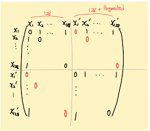
아래와 같이 mask 행렬이 구축됩니다. 즉 $x_{i} - x_{i}, x_{i} - x_{j}$ 끼리의 pair는 모두 0으로 masking으로 해준 것을 의미합니다.
그 다음 코드를 살펴보겠습니다.
z = torch.cat((z_i, z_j), dim=0)
sim = self.similarity_f(z.unsqueeze(1), z.unsqueeze(0)) / self.temperature

z_i.shape ## torch.Size([128,64])
z_j.shape ## torch.Size([128,64])

## 우선 저걸 concatenate를 함으로써 z라는 feature를 도출한다.
z.shape ## torch.Size([256,64])
우선 $z_{i}, z_{j}$는 각각 projection-head를 통해 뽑아낸 최종 feature를 의미하고 여기서는 128 배치 별 64 size의 1-dim vector를 통해 값을 추출하였습니다. 그리고 저 두 벡터를 concat한 $z$ vector를 도출합니다.
그리고 이를 다음과 같은 cosine similarity를 계산함으로써, similary matrix를 구축합니다.
## z_i, z_j 둘 사이의 cosine_similarity 계산
sim = similarity_f(z.unsqueeze(1), z.unsqueeze(0)) / temperature
저 similary는 아래 loss의 빨간 박스 부분에 해당합니다.
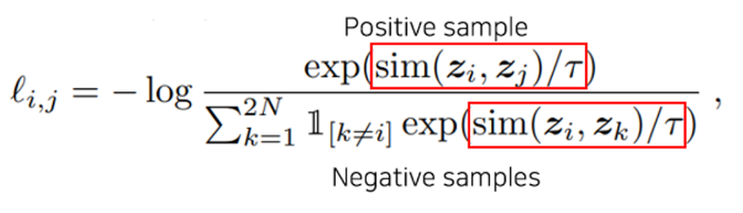
저렇게 계산한 sim matrix는 총 [256,256] 사이즈의 matrix이며 이는 각각 similarity score를 담고 있는 매트릭스가 됩니다.
sim.shape ## torch.Size([256, 256])

sim
'''
tensor([[2.0000, 1.8524, 1.7404,  ..., 1.8142, 1.8774, 1.6671],
        [1.8524, 2.0000, 1.7501,  ..., 1.7227, 1.7881, 1.5425],
        [1.7404, 1.7501, 2.0000,  ..., 1.8417, 1.7550, 1.7962],
        ...,
        [1.8142, 1.7227, 1.8417,  ..., 2.0000, 1.8388, 1.9141],
        [1.8774, 1.7881, 1.7550,  ..., 1.8388, 2.0000, 1.7453],
        [1.6671, 1.5425, 1.7962,  ..., 1.9141, 1.7453, 2.0000]],
       device='cuda:0', grad_fn=<DivBackward0>)
'''
자 그 다음 코드를 살펴보겠습니다.
sim_i_j = torch.diag(sim, batch_size * world_size)
sim_j_i = torch.diag(sim, -batch_size * world_size)

sim_i_j.shape ## torch.Size([128])
sim_j_i.shape ## torch.Size([128])
이 명령어의 경우 그림으로 표현하면 아래 매트릭스에서 다음 성분을 추출함을 의미합니다.
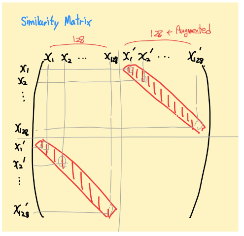
즉, 자기 자신을 제외한 positive pair 간의 similarity score를 나타내는 것이 바로 sim_i_j, sim_j_i가 됩니다. 행렬은 대칭행렬이므로 이 둘의 값은 동일합니다.
그리고 이를 다음 코드를 통해 positive pair들의 정보를 구축합니다.
positive_samples = torch.cat((sim_i_j, sim_j_i), dim=0).reshape(N, 1)
positive_samples.shape ## torch.Size([256, 1])
'''
128을 augment해서 256, 2배로 만들 때, positive pair는 그 중의 오직 한 쌍이므로,
중복 포함해서 [256,1]개가 된다 (x_i, x_j) , (x_j, x_i) 따로 세기 때문에!
이는 앞에서 대칭성을 가지고 NT-Xent loss를 계산한 것과 연결된다.
'''
그러면 이제 256개 중에서 위의 mask를 참고해서 (자기자신과 positive pair를 제외한 1로 label된 matrix, 위에서 계산한 mask ) 남은 부분이 전부 negative가 되므로 negative samples은 아래와 같이 구축됩니다.
negative_samples = sim[mask].reshape(N, -1)
negative_samples.shape ## torch.Size([256, 254]), (x_i,x_j),(x_j,x_i)2개를 제외한 254개
자 이제, 이렇게 계산을 한 positive, negative sample들의 similarity scores들을 활용해서 loss를 구축합니다.
## 여기는 positive samples들에 해당하는 수에 대응되는 label을 설정함.
## 즉, positive sample은 0, negative sample은 1로 labeling을 수행한다.
labels = torch.zeros(N).to(positive_samples.device).long()
labels.shape ## torch.Size([256])
다음과 같이 positive sample에 대한 label (0)을 구축하고 이를 바탕으로 cross entropy loss를 계산합니다.
logits = torch.cat((positive_samples, negative_samples), dim=1)
logits.shape ## torch.Size([256, 255])
'''
즉, 256개의 샘플 중에서 자기 자신을 제외하고 positive pair 1쌍과 + 남은 negative pair 254쌍이 합쳐진
[256,255]의 similarity score 값을 logit으로 설정
'''
### 저 logits을 바탕으로 cross entropy loss를 계산
CE = nn.CrossEntropyLoss(reduction="sum")
loss = CE(logits, labels)
loss /= N ## 마지막으로 1/N 을 해주면 NT-Xent loss가 계산된다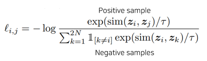
바로 저기서 logits 값을 바탕으로, entorpy 값을 계산하면 위 공식과 같고 이를 cross entropy loss를 계산하면 위와 같이 -log가 붙음으로서 최종 loss가 계산됩니다. 이를 모든 i, j pair에 대해 수행하고 마지막으로 1/N을 곱해주어 최종 loss가 계산됩니다.
결국 SimCLR는 어떠한 label (강아지+고양이..) 이 사용되지 않고 augmentation을 활용한 positive-negative sample을 바탕으로 contrastive learning을 통해 supervised learning 못지 않은 represenation 학습을 잘 수행하는 아이디어를 제안합니다. 이 아이디어는 많은 연구 분야에 사용되고 있으니 구현방법과 아이디어를 잘 숙지하면 유용할 거 같습니다.


